Diabetic Retinopathy Detection
To-Do:
- add technical overview: quote text from Gargeya’s study & recreate in code
- add references/citations
- add estimated reading time, sharing functions
Introduction
No prior knowledge is required for this article!
- In the Overview, we break down the basics of deep learning and image recognition. We’ll talk about the core concept, the math involved and how a basic model is made. Specifically, we’ll focus on the model that Gargeya & Leng use in their highly-cited paper “Automated Identification of Diabetic Retinopathy Using Deep Learning”.
- The pertinent clinical takeaways are outlined in the Key Takeaways section.
- In the Technical Overview, we dive under the hood to see how a basic model is trained with code! (coming soon).
Overview
In identifying diabetic retinopathy (DR), we traditionally interpret the retinal fundus, looking for characteristics like microaneurysms, neovascularisation and hard exudates. We’ll explore how a model can accurately detect diabetic retinopathy without explicitly knowing that information.
The Basic Concept
Broadly speaking, we’re turning data (the fundal image) into data (a number saying if DR is present or not). The fundal image is itself made out of pixels, which are numbers.
Here is information about 1 pixel in a zoomed in fundal picture. 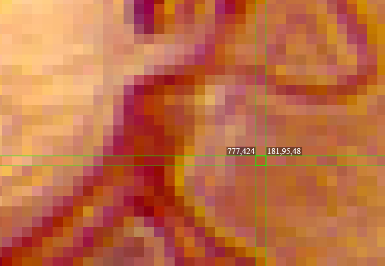
The values on the left (777 and 424) refer to the coordinates of the pixel. The values on the right refer to its “Red, Blue, Green” (RGB) values - how red, blue and green the pixel is out of a maximum of 255. Understandably, the fundus is more red than blue or green (181,95,48).
This is what it would look like if we split up the 3 colour channels. 
But the main point is that an image is simply numbers! For simplicity’s sake, let’s assume there is just 1 channel.
This is the essence of the whole model. 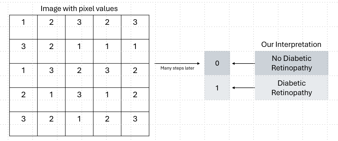
The Basic Math
We’re going to use basic addition and multiplication to turn all these pixel numbers into a final number.
The first transformation we do is called a convolution (hence these models are called convolutional neural networks).
You start off with the image matrix and a kernal (a matrix of numbers) 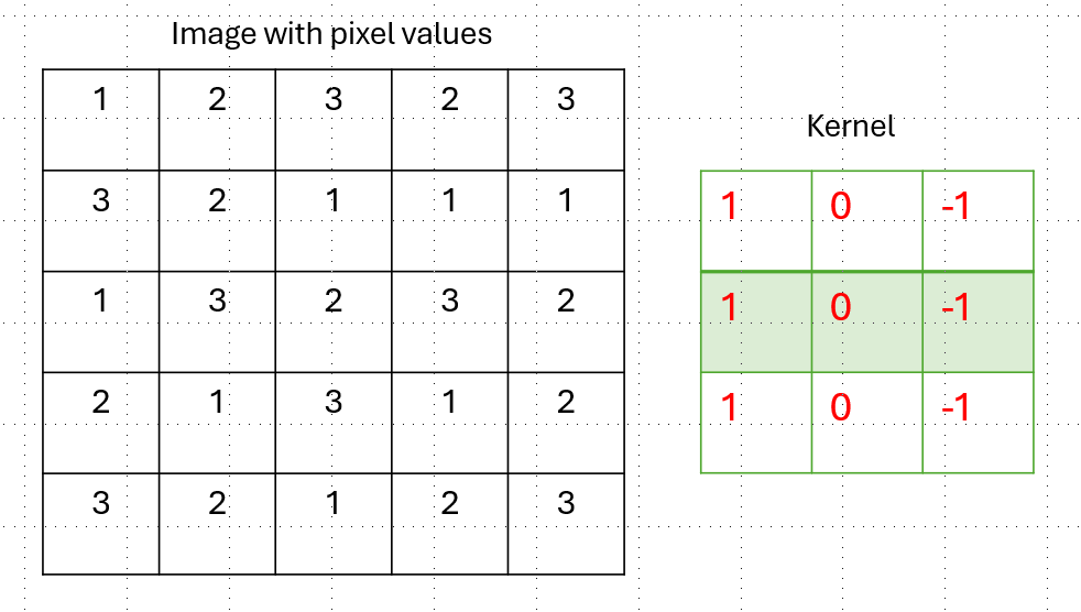
We move a kernal along the image, multiplying each kernal’s value by the pixel value and adding all of them up. 
After we apply the kernal through the image, it gives us a new matrix that we call a feature map. 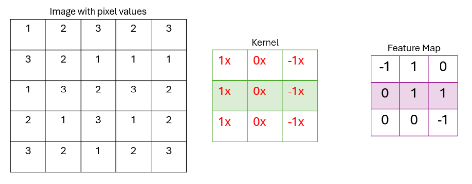
Now, why is it called a feature map? A feature map maps out key features the model uses for classification. Let’s run the number 7 from the famous MNIST database through the kernal, a large database of handwritten digits. 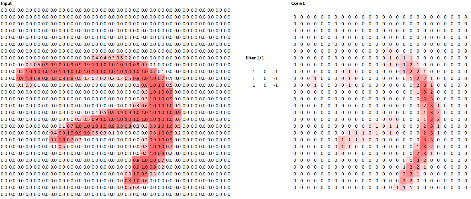
As you can see, the our feature map has highlighted the vertical parts of the image. In a sense, the model has learned what vertical lines are! Let’s use another kernal and see what happens. 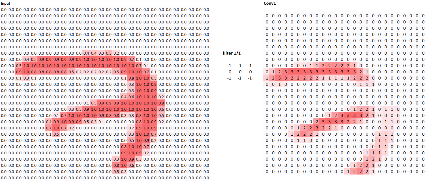
Using the multiplication and addition steps we explained above, try to see why those two kernals generate their respective feature maps!
The Basic Model
In an actual model, the original image is transformed by numerous different kernals to form a variety of feature maps. The feature maps themselves become the input to different kernals, forming new maps. This multi-layered (hence deep in ‘deep learning’) nature means complex combinations of features can be detected. The beauty of deep learning is that we don’t have to set kernals for what features we think are important - the model does that by itself. Let’s see how it does that.
The secret behind machine learning (of which deep learning is a subset of) is “gradient descent.” We’ll describe its intuition here.
Suppose I have a deep learning model that tells me if a number is 7 or not. One catch is that all of numbers in the kernals are randomised, meaning no meaningful features are being identified - our model doesn’t work. I draw the number 7 and test the model. It predicts 50-50 for if it is a 7 or not. But we know that the correct answer is 100-0 that it is a 7. Let’s say we want to improve our model so we randomly tweak the kernals. Now the model’s prediction is 60-40 in favour of 7. The model is improving!
Simply put, I want to figure out what number the kernal needs to be for our model’s prediction to be the best. This is a calculus question. With basic calculus, you can derive the direction (increase or decrease) each kernal value needs to change to improve the prediction. Now, every time our model updates its kernal values, it is improving - it is learning!
We incrementally update the kernal values, recalculating the gradient at each step so we know which direction to move in. The rate at which we change the kernals is called the learning rate (more to come on this). 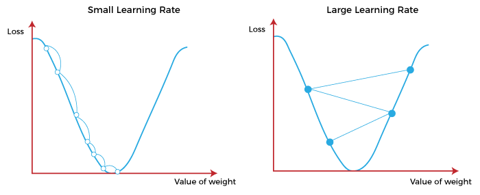
Voilà - we are now training our model! In essence, we give the model the lot of practice questions (the data) and the answer sheet (the data’s interpretation) and tell it to figure it out. This is both intelligent and not so intelligent. What if it sees a unique fundus that it has not been trained to see? Perhaps the innate features it has gathered is sufficient to remain accurate but perhaps it is not. Perhaps the dataset it is trained on is biased towards a particular demographic. Perhaps you work with a specific demographic of people and the original dataset it was trained on is too different.
This means that the training data must be heretogenous so it can work for a wide range of real-life cases. This makes it important to be critical of the sensitivity/specificity described by papers showcasing the model. Depending on the dataset the model was tested on, it may not be applicable to your patient.
You must be aware that the sensitivity/specificity described is based on a test dataset researchers have used (it varies from dataset to dataset) and ensure it is directly applicable to your patient. Here is a table from Gargeya & Leng: 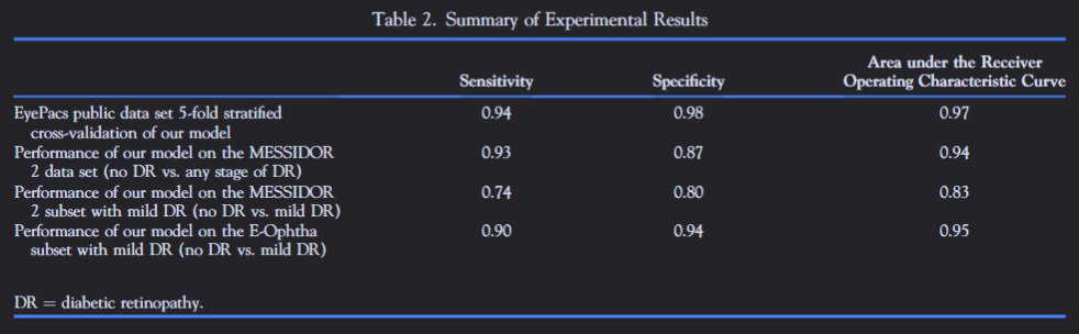 .
.
The model still performs extremely well but there is variable performance across datasets and data types (‘mild vs severe’ DR).
Key Takeaways
Deep Learning offers an extremely robust way to solve/answer any question by learning complex features invisible to us. There is an enormous variety of problems that can be solved by it (eg. risk of mortality, likelihood of falls, automation of administrative tasks, etc.)
For reliable and accurate performance, your input data must be familiar to the data the model was trained on. Therefore, data heterogenicity is important for the model’s training. This also means you might need to interpret/fix your data to be in a way the model understands (eg. the fundal image needs to be taken with roughly the same way how the model is trained)
Be aware of what datasets the model has been tested on - sufficient cross-validation is necessary to avoid bloated/overestimated specificity & sensitivity values.
Technical Overview
coming soon!
you can host models with huggingface - eg.